Introduction
We wanted to dedicate an entire post to the lovely functions cross entropy and Kullback-Leibler divergence, which are very widely used in training ML models but not very intuitive.
Luckily these two loss functions are intricately related, and in this post we’ll explore the intuitive ideas behind both, and compare & contrast the two so you can decide which is more appropriate to use in your case. We’ve also created a short interactive demo you can play around with at the bottom of the post.
Entropy
We’ll start off reviewing the concepts of information and entropy. “Information” is such an overloaded word in English, but in the statistical/information-theoretic sense, information is a quantification of uncertainty in a probability distribution. To illustrate, consider the weather. The more uncertain or random the weather seems, the more information you gain when you learn what the weather actually is. Entropy is centered around this information transfer: it’s the expected amount of information, measured in bits, in some transmission of data.

For example: suppose the weather can either be sunny or rainy.
Now suppose the true distribution of the weather is P(sunny) = ¾, P(rainy) = ¼. We could then say 00, 01, and 10 mean sunny, 11 means rainy. This is known as an encoding.
00
01
10
11
As a general rule, the information (in bits) needed to encode an outcome = \(-log_2( P(outcome) )\). Why? A singular bit can take on 2 unique values; so, if you imagine all the possible weather outcomes represented in a tree, each individual bit helps split a path in the tree in two.
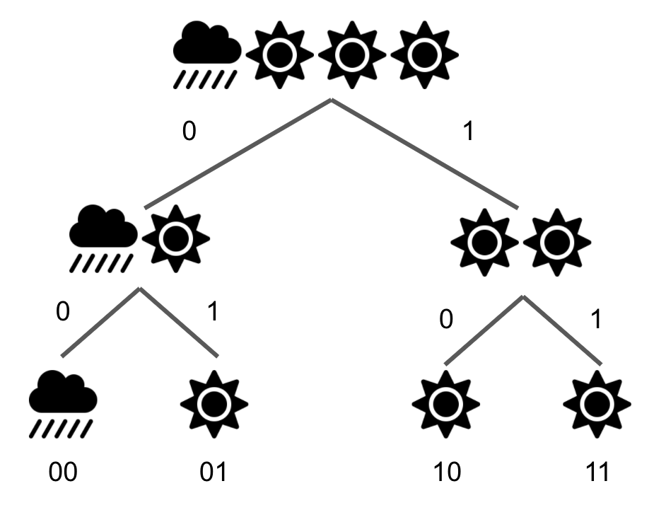
The more rare the outcome, the more information you’ll need to discern that event from others – hence the inverse relationship between probability and information for a given event. Equivalently to the above,
\[P(event) = (\frac{1}{2})^{\# bits}.\]To further illustrate this formula, let’s consider the 2 possible outcomes from learning what the weather is:
| The weather station tells us it’s rainy. We got \(-log_2(1/4)\) = 2 bits of info. The station must’ve transmitted 11, which is precisely 2 bits long. |
The weather station tells us it’s sunny. We got \(-log_2(3/4)\) = 0.415 bits of info. This is a bit trickier than the rainy case: the station transmitted one of 00, 01, or 10, which is less than 2 bits of info because we’re not certain what each bit was. |
Now to calculate the expected amount of information (entropy!), we take the weighted sum of these individual amounts of information, with weights being the probability of each outcome.
\[Entropy(weather) = H(weather) = E[Info(weather)] = P(rainy) * Info(rainy) + P(sunny) * Info(sunny)\] \[= -0.25 * log_2(0.25) - 0.75 * log_2(0.75) = 0.811.\]This tells us that given the weather follows our distribution of ¾ sunny, ¼ rainy, we’d expect that learning what the weather is for a given day (i.e., receiving the information about the weather’s value) gives us 0.811 bits’ worth of information. Or, from the other side, we expect it would take 0.811 bits to send a message saying what today’s weather was. This brings us to the general formula for entropy, which is defined for some probability distribution (in this case, of the weather) \(p\):
\[H(p) = - \sum_i p_i log_2(p_i)\]Categorical Cross Entropy
Let’s get to the main attraction: cross entropy is the expected number of bits needed to encode data from one distribution using another. So this is where our model’s prediction of the weather comes in. Maybe we live in a temperate place, so we think P(sunny) = 9/10. With our predicted distribution, this would require us to encode a “sunny” outcome with \(-log_2(9/10)\) = 0.15 bits. Since the actual probability it’s sunny is still ¾, the expected amount of information is ¾ * 0.15. So again taking the weighted sum in this manner, the formula for cross entropy loss is
\[H(p, q) = - \sum_i p_i log_2(q_i)\] \[= ¾ (0.15) + ¼ (3.32)\]Again, this represents the average number of bits needed to encode data from a source with distribution \(p\), using a model distribution \(q\). Why does this quantity of information/number of bits matter? Intuitively, the less accurate or further away \(q\) is from \(p\), the more bits are needed to represent \(p\).
When training, since we don’t know the true distribution, but instead the actual classes (labels) for individual data points, we compute the CE loss between our predicted distribution and one-hot vectors for each training point. This means a distribution with probability of 1 on the true label class, and 0 for all other classes.

For example, if our model outputted this the probability distribution
0.75
0.25
But the correct answer was sunny, making the one-hot vector:
1
0
Then the cross entropy loss is accordingly
\[- 1 * log_2(0.75) - 0 * log_2(0.25)\]Had our model predicted it was sunny with probability 1, the cross entropy loss for this example would’ve been 0. (Think about why!)

One property of the cross entropy formula is that if you predict a class has probability of 0 when its true probability is non-zero, the cross entropy loss will be infinite/undefined. This is because \(log(x)\) approaches positive infinity as x approaches 0. In practice, since we can’t backpropagate from a loss value of infinity, two solutions to this problem are
- Clip the predicted probability values at some small \(\epsilon\) value, e.g., 1e-6, which would result in a large but at least defined value.
- Clip the cross entropy loss at some large value, e.g., \(loss(p, q) = min(1000, H(p, q))\), so it never actually reaches infinity.
It’s worth noting that despite being referred to as a “distance”, cross entropy is not symmetric: \(H(p, q) \ne H(q, p)\).
Cross entropy is a great loss function to use for most multi-class classification problems. This describes problems like our weather-predicting example: you have 2+ different classes you’d like to predict, and each example only belong to one class.
The cross entropy we’ve defined in this section is specifically categorical cross entropy.
Binary cross-entropy (log loss)
For binary classification problems (when there are only 2 classes to predict) specifically, we have an alternative definition of CE loss which becomes binary CE (BCE) loss. This is commonly referred to as log loss: \(BCE(p, q) = - \sum_i p_i log(q_i) + (1 - p_i) log(1 - q_i)\)
You’ll notice that this equation has a few terms extra compared to categorical cross entropy. The \(p_i log(q_i)\) term is familiar, measuring the distance between true and predicted class probability, while the \((1 - p_i) log(1 - q_i)\) is basically the exact same penalty for the other side: we know there’s exactly 2 classes, so \((1 - p_i)\) and \((1-q_i)\) are just the probabilities for the opposite class to \(p_i\) and \(q_i\), respectively.
So when to use this instead of the categorical cross entropy loss covered above? As you may guess, this loss function is only appropriate for binary classification. Another use case would be multi-label classification, which means assigning multiple classes (“labels”) to each data point. This is essentially combining multiple binary classification tasks into one, for example, asking for a given day:
- is it rainy or not rainy?
- is it sunny or not sunny?
- is it cloudy or not cloudy?
Where the difference between this and multi-class classification is that with the former, a day can be labeled with multiple classes (e.g., rainy, not sunny, and cloudy), but for multi-class classification, only one would hold since being in one class implies not being in any other.
Kullback-Leibler (KL) divergence

KL divergence is just the difference between cross entropy and the true distribution’s entropy! \(KL(p, q) = H(p, q) - H(p)\) Rearranging terms and using log properties, we get an alternate (but more commonly seen) formulation (note that the || just signifies “distance between” in statistics): \(KL(p || q) = H(p, q) - H(p) = - \sum_i p_i log_2(q_i) - \sum_i p_i log_2(p_i) = - \sum_i p_i (log_2(q_i) - log_2(p_i)) = \sum_i p_i log(\frac{p_i}{q_i})\) which is sometimes re-expressed as: \(E[log \frac{p_i}{q_i}] = E[log p_i - log q_i]\)
Intuitively, it can be thought of as the expected number of extra bits needed to encode outcomes drawn from the true distribution \(p\) if we’re using distribution \(q\), or “the measure of inefficiency in using the probability distribution q to approximate the true probability distribution p” (thanks Wikipedia!). If we have a perfect prediction, i.e., our predicted distribution equals the true, then cross entropy equals the true distribution’s entropy, making KL divergence 0 (its minimum value).
KL divergence is used with generative models, for example, variational autoencoders (VAEs) or generative adversarial networks (GANs). At a high level, generative models generate data that follows a similar distribution as the training data (for example, https://thesecatsdonotexist.com/). KL divergence then functions as a “distance” metric between predicted and reference distribution.
See one of these awesome resources to read more:
- https://www.jeremyjordan.me/variational-autoencoders/
- https://wiseodd.github.io/techblog/2016/12/10/variational-autoencoder/
Compare n Contrast
Because the \(H(p)\) term in KL divergence doesn’t change with the predicted distribution, minimizing cross entropy (the \(H(p, q)\) term) also minimizes KL divergence. So if it seems like we’re optimizing our model in the same way using both loss functions, does it even matter which one we use?
KL divergence exactly equals cross entropy when the entropy of the true distribution is 0. This happens when there is no randomness in the distribution, i.e., one outcome/class has probability 1. Notice that this is precisely the case with how we train models, since we use a one-hot vector for the correct class. So when training a classifier for which you have some set of labelled training points you’d like your model to generalize over, the two are functionally equivalent, and you may as well just use cross entropy loss.
Meanwhile, generative models try to output a probability distribution, so KL divergence makes more sense.
So the bottom line: cross entropy is for training a classifier, KL divergence for a generator.
| Loss function | Use case(s) |
|---|---|
| Categorical cross entropy | - multi-class classification |
| Binary cross entropy | - binary classification - multi-label classification |
| KL divergence | - outputting a distribution |
Demo
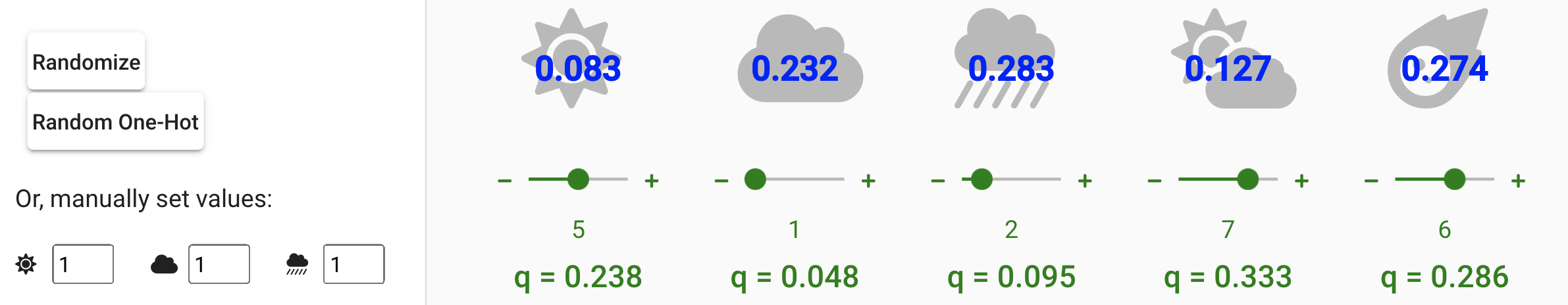
Below is the cross entropy + KL divergence demo, which uses our recurring weather classification problem. Click here for a full-screen version if preferred.
The blue text superimposed over these icons shows the true weather probability distribution, while the values shown below the classes in green are the predictions, which you can control using the sliders. As you adjust these values, you’ll see the 3 values at the bottom of the screen - entropy, cross entropy, and KL, respectively - change accordingly.
To the left of the screen is a collapsible menu. Here you can add and remove classes, up to 10 and down to 1, and change the true distribution by randomizing their values (with either a totally random distribution, or a random one-hot vector), or by manually setting the values yourself.
Note that this demo doesn’t leverage the “clipping” tricks mentioned in the section above, so setting the predicted probability to 0 for a class with non-zero true probability will result in a cross-entropy (and correspondingly, KL) of infinity!
Demo walkthrough
If you want some more guidance using the demo, click/tap the question mark button in the upper right corner, then “Play Tutorial”. This will walk you through the different things you can do with the demo and explain some of the things you see on the screen. This demo is optimized for desktop use, so if you’re reading this on a phone, I’d recommend playing with the demo on a desktop!
Let’s walk through a simple example. Make sure you have 4 classes, then click “Set” to set the true distribution to the uniform distribution (all classes have the same probability). Then set all the sliders to the same value too. Because p = q exactly, you should see that cross entropy and entropy are exactly the same. This in turn brings KL divergence down to 0, its smallest possible value. Cross entropy is also at its lowest possible value for the given problem. Now drag some sliders to change the predicted distribution to something not uniform. The farther you change it, the higher KL divergence and cross entropy will get. Now try putting your loss knowledge to the test. Toggle “Show true distribution” to hide the true distribution, then randomize it. Try to guess the true distribution by adjusting the sliders. That’s somewhat similar to how your model learns during training!